LACMIP Digitization Metrics
Overview
This document contains R code originally written to analyze the results of the “Cretaceous Seas of California” digitization project, supported by funding from the National Science Foundation (NSF DBI 1561429). The code below is designed to be reused with any dataset formatted to track daily digitization progress in the same way. A data template is available here.
If you want to re-use this code, you should open this file in R. Then begin by loading the Tidyverse library (if you haven’t already, you will also need to install the Tidyverse package):
library(tidyverse)You can also choose to redefine the following project variables:
project <- "Cretaceous Seas of California" #shows up as a graph subtitle
width <- 15 #default dimension (inches) for saving JPG versions of graphs
height <- 10 #default dimension (inches) for saving JPG versions of graphs
At this point you are ready to load the digitization time-tracking data you want to analyze into R. Edit the filename here to analyze a different dataset. Make sure your data file is in the correct working directory and formatted according to the template linked above.
data <- read_csv("input_K-CA-Digitization_2019-01-31.csv", na = character())Lots Processed
How many lots were processed as part of this project?
Use the function below to report on the number of specimen lots processed by this project.
lots <- function(data) {
#build table to summarize the number of lots processed by collection type
buildLots <- data %>%
select(matches("LOTS_")) %>%
summarise_all(funs(sum(., na.rm = TRUE))) %>%
gather("lot type","count") %>%
mutate("%" = round((count/sum(count)*100),1)) %>%
mutate(`lot type` = sub("LOTS_","",`lot type`)) %>%
mutate(`lot type` = sub("st","stratigraphic",`lot type`)) %>%
mutate(`lot type` = sub("tx","taxonomic",`lot type`))
#calculate total lots processed and
#save as an object in the global environment to access from markdown text
totalLots <<- buildLots %>%
filter(`lot type`=="stratigraphic" | `lot type`=="taxonomic") %>%
summarise(count = sum(count)) %>%
as.numeric(.[1])
#output file with results
write_csv(buildLots, "output_lots.csv")
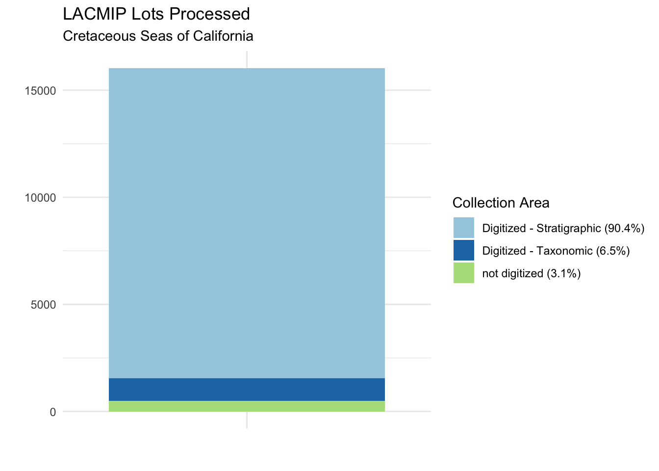
}A total of 15542 specimen lots were digitized during the Cretaceous Seas of California project. Some specimens were evaluated as part of this project but digitized, mostly due to poor quality of the original specimen. We can see a breakdown of lots processed by digitization status and collection area from the results of the function above:
Rehousing Supplies
What rehousing supplies did this project use, and at what cost?
Use the function below to report on total supplies used for this project, and their cost. Edit the values in setPrice to set different costs in dollars per unit.
supplies <- function(data) {

  #set variables for rehousing supply prices, units in dollars
  setPrice <- tibble(
    `box-3x1.5` = "0.242",
    `box-3x3` = "0.268",
    `box-3x4` = "0.372",
    `box-3x6` = "0.578",
    `box-4x6` = "0.698",
    `box-6x6` = "0.779",
    `plastic-3x3` = "1",
    `plastic-6x6` = "1",
    `vial-7dr` = "0.75",
    `vial-3dr` = "0.50",
    `vial-1dr` = "0.25")

  #turn setPrice variables into a factor
  unitPrice <- as.numeric(c(setPrice))

  #build table to calculate price per unit (note that the column names of the supplies
  #are important because the code below relies on them sorting alphabetically)
  buildSupplies <- data %>%
    select(matches("REHOUSE_")) %>%
    summarise_all(funs(sum(., na.rm = TRUE))) %>%
    gather("supply","quantity") %>%
    mutate(supply = sub("REHOUSE_box3x1.5","archival paper box, 3x1.5 inches",supply)) %>%
    mutate(supply = sub("REHOUSE_box3x3","archival paper box, 3x3 inches",supply)) %>%
    mutate(supply = sub("REHOUSE_box3x4","archival paper box, 3x4 inches",supply)) %>%
    mutate(supply = sub("REHOUSE_box3x6","archival paper box, 3x6 inches",supply)) %>%
    mutate(supply = sub("REHOUSE_box4x6","archival paper box, 4x6 inches",supply)) %>%
    mutate(supply = sub("REHOUSE_box6x6","archival paper box, 6x6 inches",supply)) %>%
    mutate(supply = sub("REHOUSE_plastic3x3","archival plastic box, 3x3 inches",supply)) %>%
    mutate(supply = sub("REHOUSE_plastic6x6","archival plastic, 6x6 inches",supply)) %>%
    mutate(supply = sub("REHOUSE_vial7dr","glass vial, 7 dram",supply)) %>%
    mutate(supply = sub("REHOUSE_vial3dr","glass vial, 3 dram",supply)) %>%
    mutate(supply = sub("REHOUSE_vial1dr","glass vial, 1 dram",supply)) %>%
    mutate("cost ($)" = round(quantity*unitPrice,2))

  #calculate total supply cost and
  #save as an object in the global environment to access from markdown text
  totalCost <<- sum(buildSupplies$`cost ($)`)

  #output file with results
  write_csv(buildSupplies, "output_supplies.csv")

}
The total cost for the Cretaceous Seas of California project was $4491.54. We can see a breakdown of costs by supply item from the results of the function above:
| supply | quantity | cost ($) |
|---|---|---|
| archival paper box, 3x1.5 inches | 929 | 224.82 |
| archival paper box, 3x3 inches | 423 | 113.36 |
| archival paper box, 3x4 inches | 206 | 76.63 |
| archival paper box, 3x6 inches | 215 | 124.27 |
| archival paper box, 4x6 inches | 169 | 117.96 |
| archival paper box, 6x6 inches | 276 | 215.00 |
| archival plastic box, 3x3 inches | 104 | 104.00 |
| archival plastic, 6x6 inches | 22 | 22.00 |
| glass vial, 7 dram | 2956 | 2217.00 |
| glass vial, 3 dram | 1296 | 648.00 |
| glass vial, 1 dram | 2514 | 628.50 |
Taxonomic Improvements
What taxonomic improvements were made during this project?
Use the function below to report on the effect that this project had on the quantity and quality of taxonomic identifications for lots processed during its course.
identifications <- function(data) {

  #build table to calculate taxonomic identification actions by type
  buildIdentifications <- data %>%
    select(matches("ID_")) %>%
    summarise_all(funs(sum(.,na.rm = TRUE))) %>%
    gather("identification action","count") %>%
    mutate(`identification action` =
      sub("ID_genusChange","genus name updated or redetermined",`identification action`)) %>%
    mutate(`identification action` =
      sub("ID_speciesChange","species name updated or redetermined",`identification action`)) %>%
    mutate(`identification action` =
      sub("ID_sp","evaluated but could not assign species name",`identification action`)) %>%
    mutate(`identification action` =
      sub("ID_rank-up","taxonomic rank moved up  ",`identification action`)) %>%
    mutate(`identification action` =
      sub("ID_rank-down","taxonomic rank moved down ",`identification action`)) %>%
    mutate(`identification action` =
      sub("ID_new","identification assigned for the first time",`identification action`)) %>%
    mutate("% total lots" = round((count/totalLots*100),1))

  #calculate the total percent of specimen lots affected by taxonomic identification action and
  #save as an object in the global environment to access from markdown text
  totalIdentifications <<- sum(buildIdentifications$`% total lots`)

  #output results as file
  write_csv(buildIdentifications, "output_identifications.csv")

}
A total of 65.3% of specimen lots had their taxonomic quality improved during the Cretaceous Seas of California project. We can see a breakdown of taxonomic improvements from the results of the function above:
| identification action | count | % total lots |
|---|---|---|
| genus name updated or redetermined | 825 | 5.3 |
| species name updated or redetermined | 239 | 1.5 |
| evaluated but could not assign species name | 60 | 0.4 |
| taxonomic rank moved up | 689 | 4.4 |
| taxonomic rank moved down | 595 | 3.8 |
| identification assigned for the first time | 7748 | 49.9 |
Digitization Rate
What was this project’s overall digitization rate?
Use the function below to report on the rate of digitization over the lifespan of this project, as measured by the number of specimen lots processed.
digitizationRate <- function(data) {

  #build table to summarize number of lots processed over time
  buildDigitizationRate <- data %>%
    select(matches("LOTS_|date")) %>%
    mutate("lots" = LOTS_st + LOTS_tx) %>%
    separate(date, c("yyyy","mm","dd"), sep = "-") %>%
    unite("month", c("yyyy","mm"), sep = "-") %>%
    select(month,lots) %>%
    na.omit() %>%
    group_by(month) %>%
    summarise(lots = sum(lots))

  #calculate the mean number of lots processed per month and
  #save as an object in the global environment to access from markdown text
  averageLots <<- mean(buildDigitizationRate$lots)

  #output results to file
  write_csv(buildDigitizationRate, "output_digitizationRate.csv")

  #graph digitization rate by month
  graphDigitizationRate <- buildDigitizationRate %>%
    ggplot(aes(x = month, y = lots)) +
    geom_col() +
    labs(title = "LACMIP Digitization Rate by Lots",
         subtitle = project,
         y = "# of Lots Processed",
         x = "\nMonth") +
    theme_minimal() +
    theme(axis.text.x = element_text(angle = 45, hjust = 1, vjust = 1))

  #output graph to file
  ggsave("output_digitizationRate.jpg", plot = graphDigitizationRate,
         width = width*1.5, height = height, units = "cm", dpi = "print")

}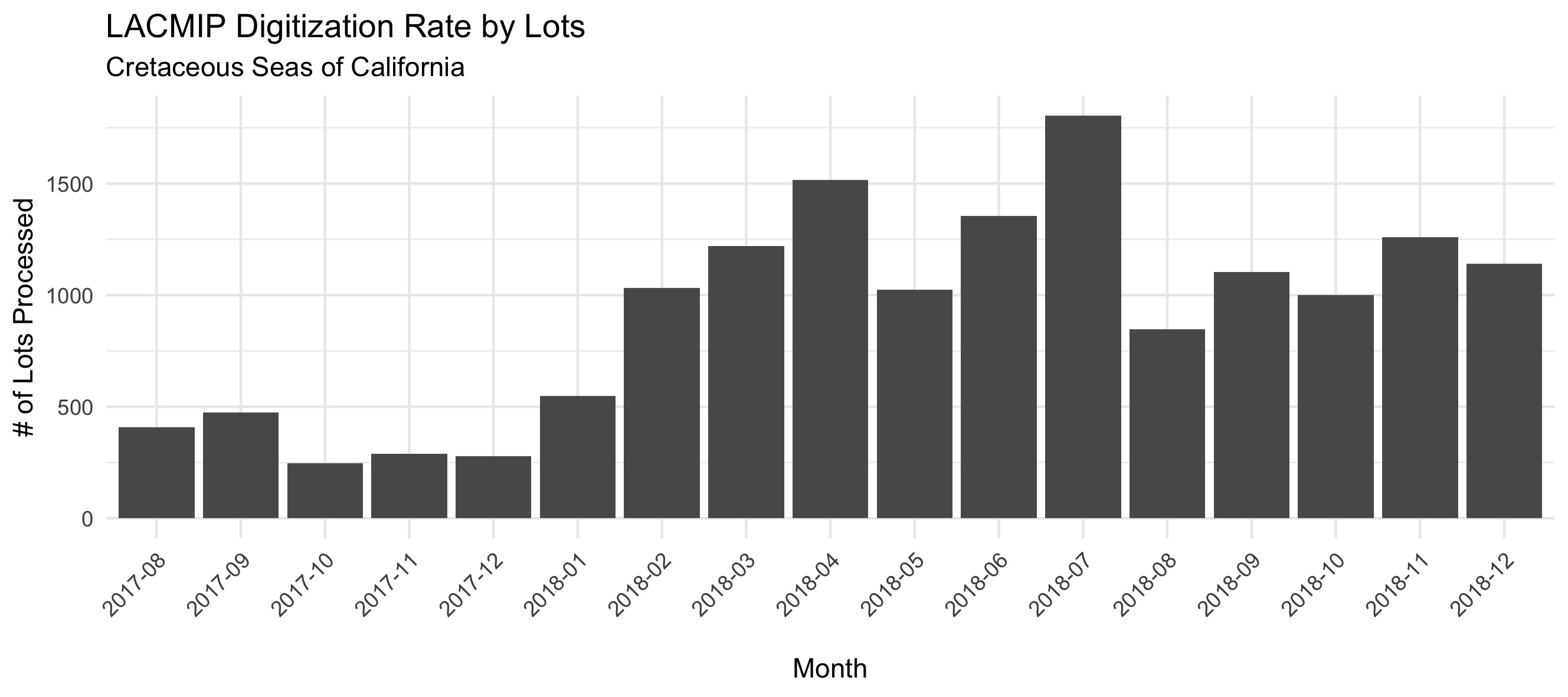
The Cretaceous Seas of California project digitization rate is graphed here by the number of lots processed over time, an average of 914 specimen lots per month.
What digitization tasks required the most time?
Use the function below to report on the time required to perform each of the core tasks associated with specimen digitization.
digitizationTask <- function(data) {
#streamline main data for task analysis
buildDigitizationTask <- data %>%
mutate(lotsProcessed = select(., matches("LOTS_"),-LOTS_uncataloged)
%>% rowSums(na.rm = TRUE)) %>%
mutate(lotsRehoused = select(., matches("REHOUSE_"))
%>% rowSums(na.rm = TRUE)) %>%
mutate(lotsIdentified = select(., matches("ID_new"))
%>% rowSums(na.rm = TRUE)) %>%
mutate(lotsReidentified = select(., matches("ID_"),-ID_new)
%>% rowSums(na.rm = TRUE)) %>%
filter(lotsProcessed!=0) %>%
mutate(minutesPerIDRehouse = round(`TIME_idRehouse`*60/lotsProcessed,1)) %>%
mutate(minutesPerCount = round(`TIME_count`*60/lotsProcessed,1)) %>%
mutate(minutesPerPaint = round(`TIME_paint`*60/lotsProcessed,1)) %>%
mutate(minutesPerCatalog = round(`TIME_catalog`*60/lotsProcessed,1)) %>%
mutate(minutesPerLabels = round(`TIME_labels`*60/lotsProcessed,1)) %>%
mutate(minutesPerNumber = round(`TIME_number`*60/lotsProcessed,1)) %>%
mutate(minutesPerTotal = select(., matches("minutesPer"))
%>% rowSums(na.rm = TRUE)) %>%
select(date, matches("LOC_"), matches("minutes"),
lotsProcessed, lotsRehoused, lotsIdentified, lotsReidentified)
#output results to file
write_csv(buildDigitizationTask, "output_digitizationTask.csv")
#calculate average minutes per specimen lot per task
buildDigitizationTaskAvg <- tibble(
"Task" = c("Identify & Rehouse", "Count", "Paint", "Catalog", "Place Labels", "Number"),
"Time (min/lot)" = c(round(mean(buildDigitizationTask$minutesPerIDRehouse, na.rm = TRUE),1),
round(mean(buildDigitizationTask$minutesPerCount, na.rm = TRUE),1),
round(mean(buildDigitizationTask$minutesPerPaint, na.rm = TRUE),1),
round(mean(buildDigitizationTask$minutesPerCatalog, na.rm = TRUE),1),
round(mean(buildDigitizationTask$minutesPerLabels, na.rm = TRUE),1),
round(mean(buildDigitizationTask$minutesPerNumber, na.rm = TRUE),1)))
#calculate average minutes per specimen lot (all tasks) and
#save as an object in the global environment to access from markdown text
averageTimePerLot <<- sum(buildDigitizationTaskAvg$`Time (min/lot)`)
#graph average minutes per specimen lot per task
graphDigitizationTaskAvg <<- buildDigitizationTaskAvg %>%
ggplot(aes(x = Task, y = `Time (min/lot)`, label = `Time (min/lot)`)) +
geom_bar(stat = "identity") +
scale_x_discrete (limits = c("Identify & Rehouse","Count",
"Catalog","Paint","Number","Place Labels")) +
labs(title = "LACMIP Digitization Time per Task",
subtitle = project,
y = "Average Time per Lot (minutes)",
x = "\nTask") +
theme_minimal() +
geom_text(vjust = 0, nudge_y = 0.05)
#output graph to file
ggsave("output_digitizationTaskAvg.jpg", plot = graphDigitizationTaskAvg,
width = width, height = height, units = "cm", dpi = "print")
#calculate average minutes per specimen lot per task over time
buildDigitizationTaskTime <- buildDigitizationTask %>%
select(date, starts_with("minutes")) %>%
gather("task","time",-date, na.rm = TRUE) %>%
group_by(date, task) %>%
mutate(minutesPerSpm = round(mean(time, na.rm = TRUE),1)) %>%
ungroup() %>%
mutate(task = sub("minutesPer","",task)) %>%
select(-time) %>%
distinct()
#[FIX] set factor to order tasks according to natural sequence
#buildDigitizationTaskTime$task2 = factor(buildDigitizationTaskTime$task, levels =
# c("IDRehouse","Count","Catalog","Paint","Number","Labels"))
#graph average minutes per specimen lot per task over time
graphDigitizationTaskTime_task <<- buildDigitizationTaskTime %>%
spread(task, minutesPerSpm) %>%
select(-Count, -Total) %>%
filter_all(all_vars(!is.na(.))) %>%
gather("task", "minutesPerSpm", -date) %>%
ggplot(aes(x = as.factor(date), y = minutesPerSpm, group = task, color = task)) +
geom_line() +
#coord_cartesian(ylim = c(0, 40)) +
facet_grid(rows = vars(task), scales = "free") +
labs(title = "LACMIP Digitization Rate by Task",
subtitle = project,
y = "Average Time per Lot (minutes)",
x = "\nProject Duration") +
theme_minimal() +
theme(axis.text.x = element_blank())
#output graph to file
ggsave("output_digitizationTaskTime_task.jpg", plot = graphDigitizationTaskTime_task,
width = width*1.5, height = height, units = "cm", dpi = "print")
#graph average minutes per specimen lot (all tasks) over time
graphDigitizationTaskTime_total <<- buildDigitizationTaskTime %>%
filter(task == "Total") %>%
ggplot(aes(x = date, y = minutesPerSpm)) +
geom_point() +
geom_smooth() +
labs(title = "LACMIP Digitization Rate by Time per Lot",
subtitle = project,
y = "Average Time per Lot (minutes)",
x = "\nProject Duration") +
theme_minimal() +
theme(axis.text.x = element_text(angle = 45, hjust = 1, vjust = 1))
#output graph to file
ggsave("output_digitizationTaskTime_total.jpg", plot = graphDigitizationTaskTime_total,
width = width*1.5, height = height, units = "cm", dpi = "print")
#[FIX TITLE] calculate average minutes per specimen lot per task over time
#buildDigitizationTaskFactor <-
#graph average minutes per specimen lot (all tasks) over time, faceted by formation
#graphDigitizationTaskFactor <<-
#output graph to file
#ggsave("output_digitizationFactor_formation.jpg", plot = graphDigitizationFactor_formation,
# width = width*1.5, height = height, units = "cm", dpi = "print")
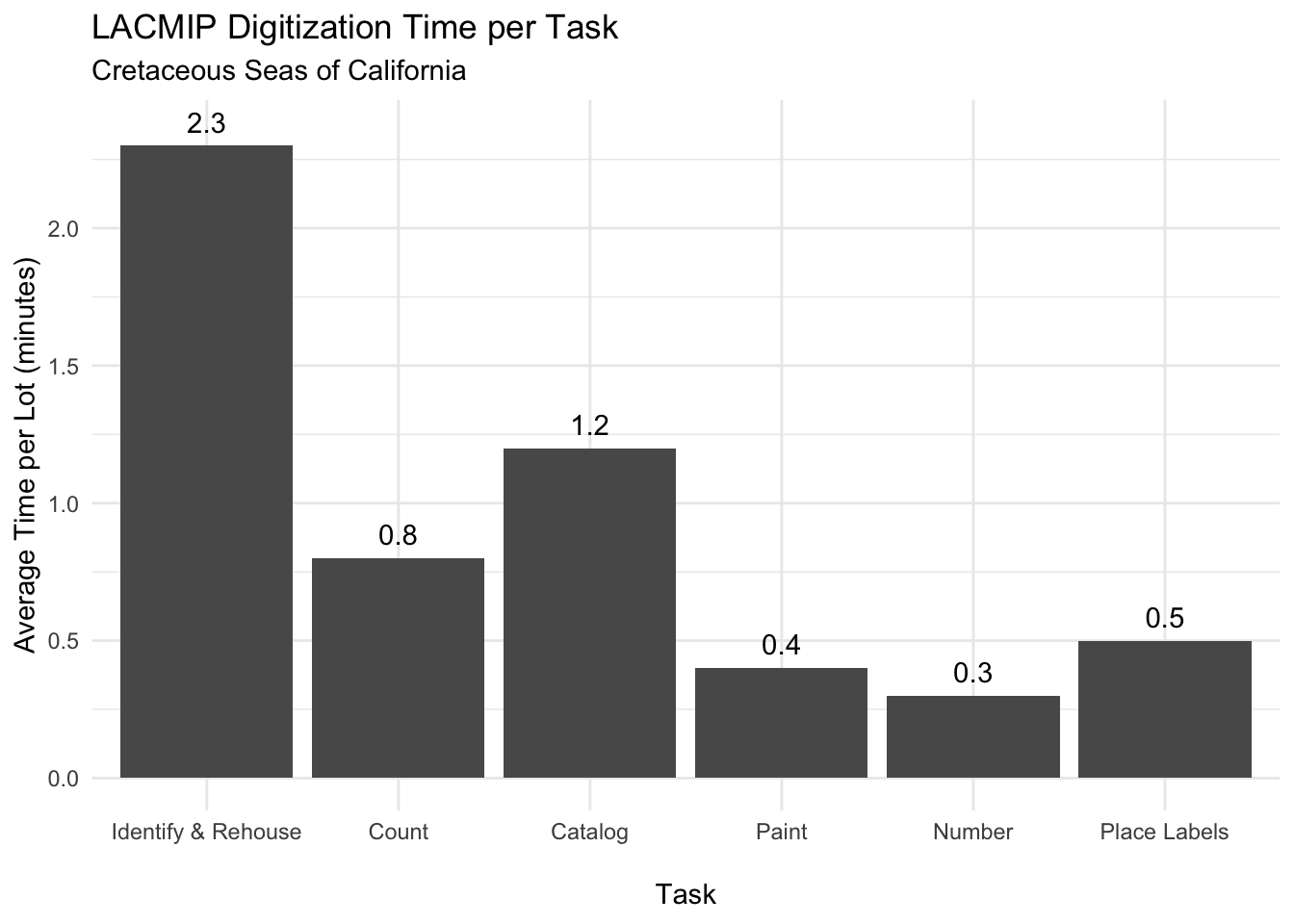
}Digitization is comprised of specific tasks, often completed by people with different roles in the project (staff, student, volunteer, etc.). LACMIP identified and tracked six specific digitization tasks, and the average time required to complete each task for one specimen lot is graphed here:
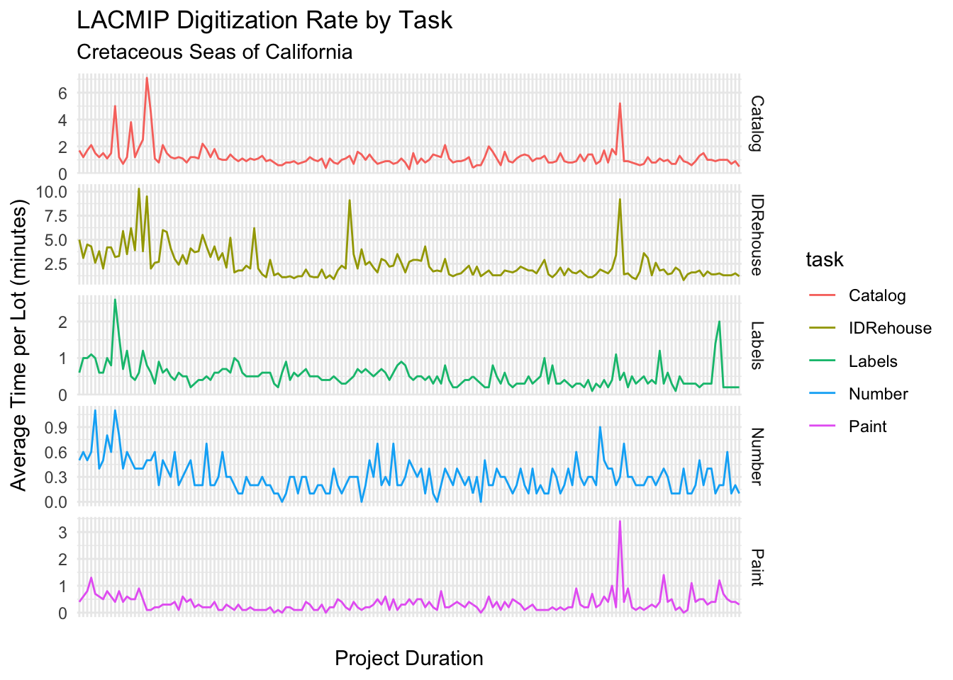
The digitization rate over time broken up by task is graphed here:
What factors affected digitization rates?
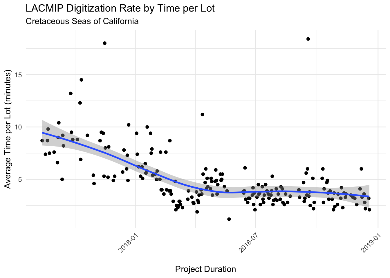
The average time to digitize a single specimen lot (all tasks included) varied, as shown in the graph here, clearly indicating that overall project duration affected digitization rate. Over the course of the project as a whole, each specimen lot took an average of 5.5 minutes per lot to process.